4749

Sparse DCE-MRI using a Temporal Constraint Learned from Clinical Data

Sreedevi Gutta¹, Yannick Bliesener¹, Jay Acharya², Meng Law², and Krishna S. Nayak^1,2

¹Electrical Engineering, University of Southern California, Los Angeles, CA, United States, ²Radiology, University of Southern California, Los Angeles, CA, United States

Synopsis

Dynamic contrast enhanced MRI has benefitted substantially from developments in sparse sampling and constrained reconstruction. Thus far, temporal constraints have proven to be the most powerful. In this work, we explore the use of temporal dictionaries that are learned from a clinical database. We demonstrate that this method provides improved reconstruction quality compared to state-of-the-art TK-model-based constraints or low-rank constraints. The inclusion of spatial information while constructing dictionaries is also explored.

INTRODUCTION

Dynamic contrast enhanced (DCE) MRI involves intravenous injection of a T₁-shortening contrast agent followed by the repeated acquisition of T₁ weighted images providing measurements of signal enhancement as a function of time¹. The dynamic anatomic images are then utilized to estimate tracer-kinetic (TK) parameters such as vascular permeability and fractional plasma volume for each voxel². Standard methods are unable to simultaneously provide high spatiotemporal resolution and volume coverage³. DCE has experienced major improvements through the use of sparse data sampling⁴. Parallel imaging (PI) and constrained reconstruction techniques have all been used to provide substantial improvements in resolution and coverage^5-7. Recently, a model-based reconstruction that imposes TK model as a consistency constraint was developed for DCE imaging and has enabled the highest under-sampling rates to date⁸. However, this method may suffer from model inconsistencies and inaccurate arterial input function extraction. Here, we investigate dictionary learning (DL) algorithm that learns temporal constraint from clinical DCE-MRI data. We found this technique provides improved performance compared to global low rank (GLR)⁹ or model consistency (MOCCO)⁸ constraint.

METHODS

DL involves finding a basis set that is optimal for a specific set of signals to provide the sparsest possible representation for that particular signal¹⁰. The reconstruction problem can be expressed as the following optimization:

m i n_{D, α, s (r, t)} \sum_{i} | | α_{i} | |_{0} + \sum_{c} | | F_{u} C_{c} (r) s (r, t) - S_{c} (k, t) | |_{2}^{2}

$min_{D,\alpha,s(r,t)} \sum_i ||\alpha_i||_0 + \sum_c ||F_u C_c(r)s(r,t) - S_c(k,t)||_2^2$

s . t | | P_{i} (s (r, t)) - D α_{i} | |_{2}^{2} < ϵ \forall i

$s.t \quad ||P_i(s(r,t)) - D \alpha_i||_2^2 < \epsilon \quad \forall \quad i$

where $s(r,t)$ are dynamic anatomic images, $C_c(r)$ are the coil-sensitivities estimated using sum-of-squares coil combination, $S_c(k,t)$ is the under-sampled $(k,t)$ space data with $k$ representing the $k$ -space coordinates, $r$ denoting the image domain spatial coordinates, $c$ and $t$ are the coil and time dimensions, $F_u$ is the under-sampling Fourier transform, $D$ is the learned dictionary, $\alpha$ is the sparse representation, $||.||_0$ counts the number of non-zero elements, and $P_i$ is an operator that extracts 3D patches as a column vector. The optimization problem is non-convex and can be solved by splitting into two simpler subproblems. Iteratively solving these two subproblems will yield an approximate solution. Results were compared against GLR, MOCCO, and the fully-sampled reference. A fixed number of iterations was empirically chosen for both DL and GLR based on convergence behavior in retrospective under-sampling studies.

. First, we assume $s(r,t)$ is fixed while $D$ and $\alpha$ are free variables. This step finds a dictionary that can sparsely represent the dataset using k-SVD algorithm¹⁰. The trained dictionary is later used to sparsely code the dataset using orthogonal matching pursuit (OMP)¹¹.

. The second step is data consistency, in which $s(r,t)$ is the only free variable. In this step, we insert the measured data at the sampling locations.

The datasets used in this study were from brain tumor patients receiving a routine brain MRI with contrast on a clinical 3 Tesla scanner at our institution. A 3D cartesian fast SPGR sequence with field of view (FOV): $22\times22\times4.2 cm^3$ ; spatial resolution: $0.9\times1.3\times7.0 mm^3$ ; temporal resolution: 5 seconds; 50-time frames; 8 receiver coils; $15^{\circ}$ flip angle; 1.3 ms echo time; and 6 ms TR was used. A dictionary of 800 elements was trained using 768000 patches from 20 fully-sampled datasets. This dictionary was then used to reconstruct 15 test datasets (retrospectively down-sampled).

RESULTS AND DISCUSSION

Reconstruction time was: GLR ~0.55 minutes for 50 iterations; MOCCO ~5.33 minutes; DL ~23.74 minutes for training and ~7.15 minutes for reconstruction with 20 iterations. The major computational burden is the sparse coding step, which takes ~ 6.67 minutes for 20 iterations.

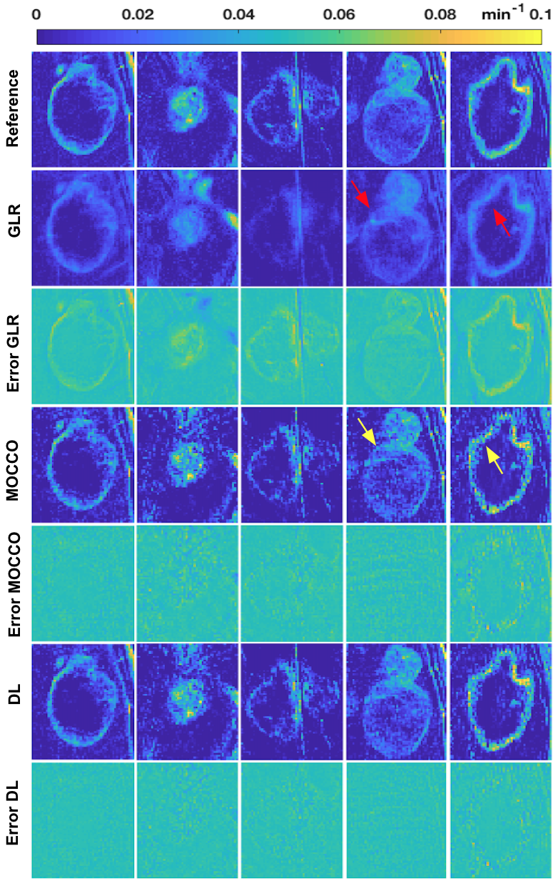
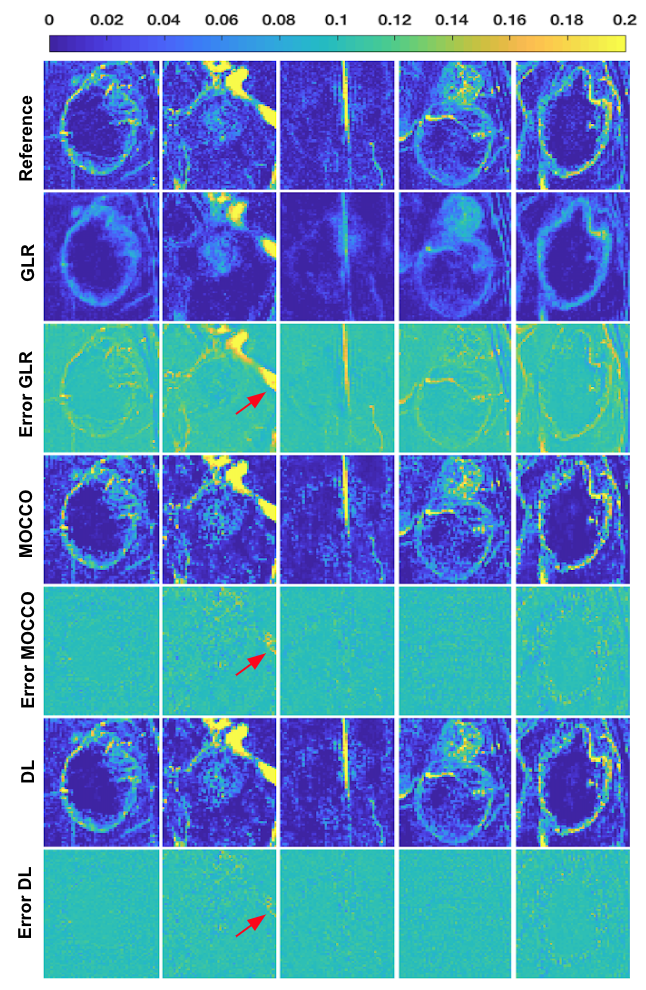
Figure 1 contains tumor $k^{trans}$ ROI maps for 5 representative tumors (out of 15) for an under-sampling rate of 40 in the testing dataset. Figure 2 shows matching tumor $v_p$ ROI maps. TK maps reconstructed from GLR appear spatially smooth and those from MOCCO show a higher noise level.

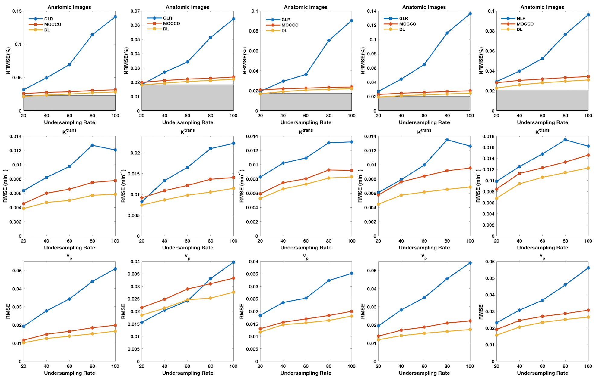
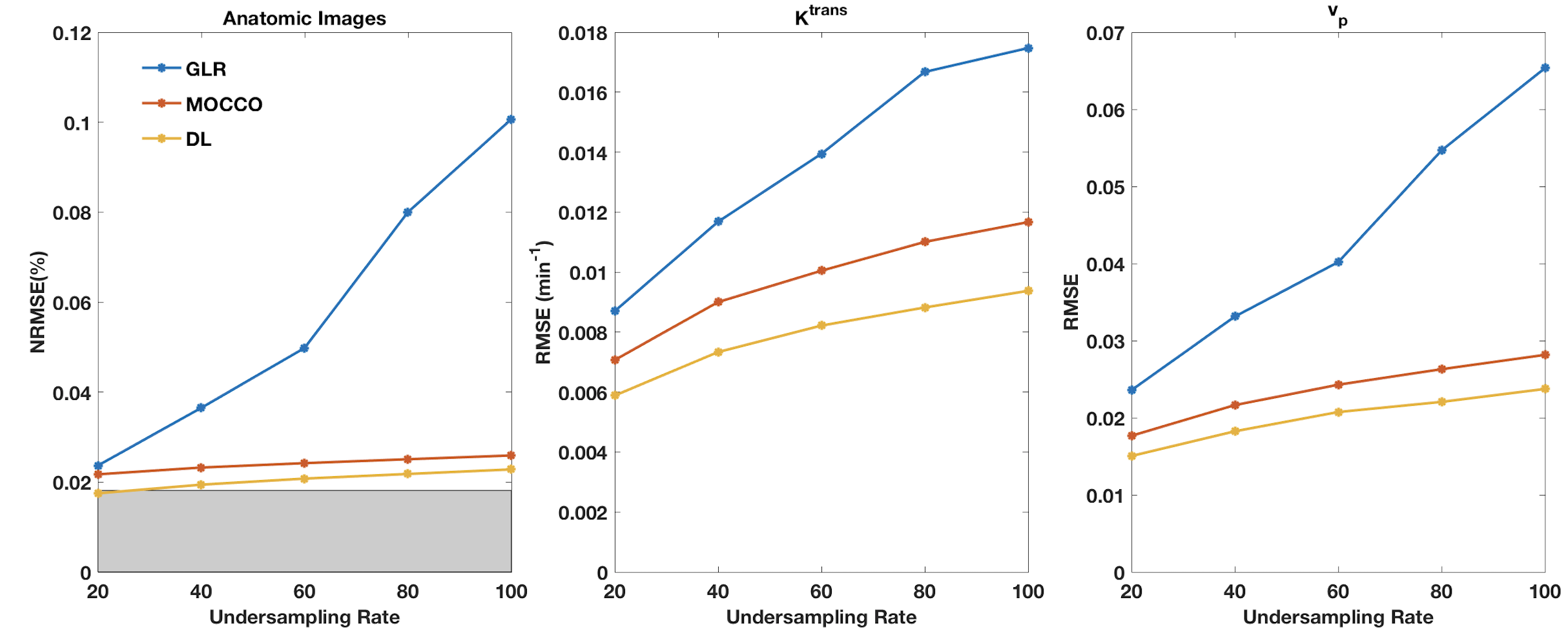
Figure 3 compares the performance as a function of under-sampling. Each column corresponds to the tumors shown in Figs. 1 and 2. DL consistently provided lower NRMSE compared to the alternatives that were studied. Figure 4 shows the average RMSE for all 15 tumors in the test dataset. The improvement of DL with respect to GLR is significant, whereas the improvement with respect to MOCCO is minimal.

We also explored the use of spatio-temporal dictionaries (not shown here), and these provided significant denoising. This warrants further exploration along with a comparison to previous spatio-temporal constraints.

CONCLUSION

Sparse DCE-MRI reconstruction using a learned temporal constraint from clinical data may outperform current temporally constrained methods. The proposed technique was evaluated on 15 brain tumor cases and provided superior performance in every case.

Acknowledgements

We acknowledge National Institute of Health grant support (#R33-CA225400).

References

1. Heye AK, Culling RD, Hernandez MD, et al. Assessment of blood–brain barrier disruption using dynamic contrast-enhanced MRI. A systematic review. Neuroimage Clin. 2014;6:262-274.

2. Sourbron SP, Buckley DL. Classic models for dynamic contrast‐enhanced MRI. NMR Biomed. 2013;26(8):1004-1027.

3. Planey CR, Welch EB, Xu L, et al. Temporal sampling requirements for reference region modeling of DCE-MRI data in human breast cancer. J Magn Reson Imaging. 2009;30(1):121-134.

4. Paldino MJ, Barboriak DP. Fundamentals of quantitative dynamic contrast-enhanced MR imaging. Clin North Am. 2009;17(2):277-289.

5. Tudorica LA, Oh KY, Roy N, et al. A feasible high spatiotemporal resolution breast DCE-MRI protocol for clinical settings. Magn Reson Imaging. 2012;30(9):1257-1267.

6. Lustig M, Donoho D, Pauly JM. Sparse MRI: the application of compressed sensing for rapid MR imaging. Magn Reson Med. 2007;58(6):1182-1195.

7. Lebel RM, Jones J, Ferre JC, et al. Highly accelerated dynamic contrast enhanced imaging. Magn Reson Med. 2014;71(2):635-644.

8. Guo Y, Lingala SG, Bliesener Y, et al. Joint arterial input function and tracer kinetic parameter estimation from undersampled dynamic contrast‐enhanced MRI using a model consistency constraint. Magn Reson Med. 2018;79(5):2804-2815.

9. Zhang T, Pauly JM, Levesque IR. Accelerating parameter mapping with a locally low rank constraint. Magn Reson Med. 2015;73(2):655-661.

10. Aharon M, Elad M, Bruckstein A. K-SVD: An algorithm for designing overcomplete dictionaries for sparse representation. IEEE Trans. Signal Process. 2006;54(11):4311-4322.

11. Tropp JA, Anna, and Gilbert C. Signal recovery from random measurements via orthogonal matching pursuit. IEEE Trans. Inf. Theory. 2007;53(12):4655-4666.

Figures

Figure 1: Brain tumor

k^{t r a n s}

$k^{trans}$ maps from 5 (out of 15) representative cases for an under-sampling rate of 40. Top row contains reference maps obtained from fully-sampled data, followed by GLR, error between reference and GLR, MOCCO, error between reference and MOCCO, DL, and error between reference and DL. In general, GLR reconstructions appear excessively smooth (red arrows) and MOCCO reconstructions appear noisy (yellow arrows).

Figure 2: Brain tumor

v_{p}

$v_p$ maps from 5 (out of 15) representative cases for an under-sampling rate of 40. Top row contains reference maps obtained from fully-sampled data, followed by GLR, error between reference and GLR, MOCCO, error between reference and MOCCO, DL, and error between reference and DL. In general, DL results were comparable to MOCCO, and sharper than GLR (red arrows).

Figure 3: RMSE for the tumor ROI as a function of under-sampling rate for the 5 tumor cases (each column) shown in Fig. 1 and 2. (top) Anatomic images; (middle)

k^{t r a n s}

$k^{trans}$ ; (bottom)

v_{p}

$v_p$ . The DL method with temporal dictionary has reduced NRMSE compared to GLR and MOCCO at all under-sampling factors varying from 20 to 100. The NRMSE due to thermal noise in the fully sampled reference is shown as the shaded gray region. This indicates that the improvement with respect to GLR is substantial, but the improvement with respect to MOCCO is minor.

Figure 4: Average RMSE across 15 cases as a function of under-sampling rate. (left) Anatomic images; (middle)

k^{t r a n s}

$k^{trans}$ ; (right)

v_{p}

$v_p$ . The NRMSE due to thermal noise in the fully sampled reference is shown as the shaded gray region. This indicates that the improvement with respect to GLR is substantial, but the improvement with respect to MOCCO is minor.

Proc. Intl. Soc. Mag. Reson. Med. 27 (2019)

4749