0673
Calibrationless Deblurring of Spiral RT-MRI of Speech Production Using Convolutional Neural Networks1University of Southern California, Los Angeles, CA, United States
Synopsis
Spiral acquisitions are preferred in speech real-time MRI because of their high efficiency, making it possible to capture vocal tract dynamics during natural speech production. A fundamental limitation is signal loss and/or blurring due to off-resonance, which degrades image quality most significantly at air-tissue boundaries. Here, we present a machine learning method that corrects for
Introduction
Blurring and/or signal loss due to off-resonance is the primary limitation of spiral MRI. When applied to speech real-time MRI (RT-MRI), this degrades image quality most significantly at air-tissue boundaries, which are the exact locations of interest.1–3 Inspired by multi-frequency interpolation (MFI)4 and in the light of recent convolutional neural network (CNN) methods,5–7 we consider a CNN network that directly learns an end-to-end mapping between distorted and residual (distortion-free minus distorted) images for 1.5T spiral speech RT-MRI.Methods
Network Architecture
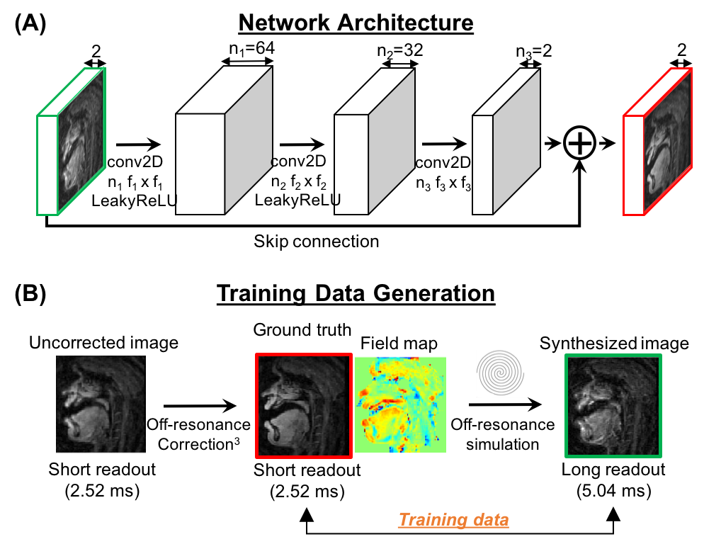
Figure 1(A) illustrates the proposed network architecture, inspired by the concept of MFI. The network is composed of 3 convolution layers: the first layer applies 2D convolutions to its input, followed by LeakyReLU, which is analogous to reconstructing base images at several demodulation frequencies in MFI. The second layer applies 2D convolutions with 1x1 spatial support and LeakyReLU activation to its input. The last layer has a 2D convolution unit without activation. These latter two layers are analogous to spatially-varying weighting and summation in MFI. Unlike MFI, which uses a linear mapping derived from a field map, the machine learning approach trains a non-linear mapping from training data. We also consider a residual CNN by introducing a skip connection from input to output to improve deblurring performance. Both the input and output of the networks consist of two channels for real and imaginary components. Tensorflow8 was used for the implementation.
Training Data
We used datasets of 29 subjects for the training and validation sets. Training data were generated from 7200 images of 18 subjects (each with 400 time frames) acquired with short spiral readout (2.52ms) on a 1.5 T GE scanner.3 As illustrated in Figure 1(B), ground truth images were obtained from the short readout images after off-resonance correction.3 For distorted images, off-resonance was simulated from the ground truth using a long readout (5.04ms) spiral trajectory and field maps estimated from the correction step. The original field map values were scaled by (1, 2/3, 1/3, 1/6) to yield different maximum off-resonance frequency ranges (fmax = ± 625, ± 417, ± 208, ± 125 Hz), corresponding to phase accrual of 3.15, 2.1, 1, 0.63 cycle/readout. Datasets from 11 human subjects were separately used as the validation set.
Experiments
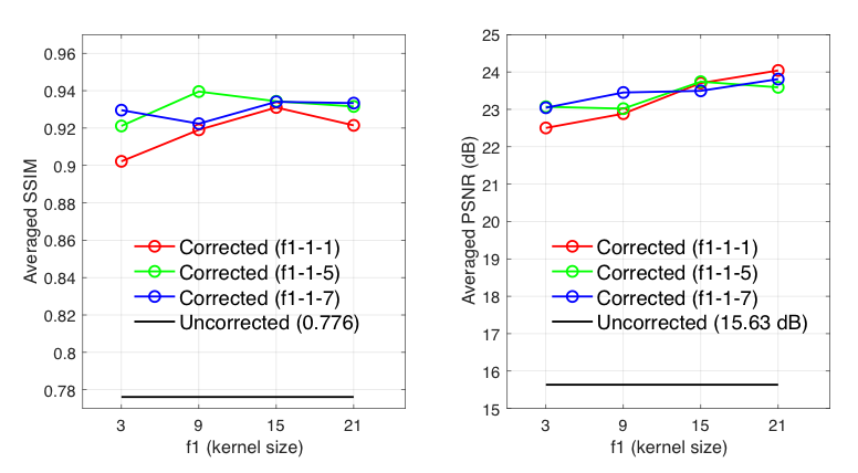
We investigate the network sensitivity to filter size, f1 and f3 of the first and third convolution layers. The full-width-half-maximum of the point spread function at 3 cycles per readout is approximately 21 pixels. Thus, we varied f1 up to this upper limit such that f1 = {3, 9, 15, 21}. We also varied f3 = {1, 5, 7}, but fixed f2 = 1 for all studies. We also examine the impact of off-resonance frequency range in the training data on the deblurring performance. Specifically, while keeping other parameters constant, we train the network on data simulated with the 4 different fmax at a time and compare its model performance on validation data. Finally, spiral dynamic images acquired with longer readouts (2.52, 4.016, 5.320, 7.936ms) were deblurred frame-by-frame by the trained network and the results were compared with a recent dynamic off-resonance correction method.3
Results and Discussion
Figure 2 shows that deblurring performance tends to improve (but not always) as f1 and f3 increase. We expect there should be a point where performance starts to degrade; this remains to be explored. We chose f1-f2-f3 = 15-1-5 for the rest of this study.
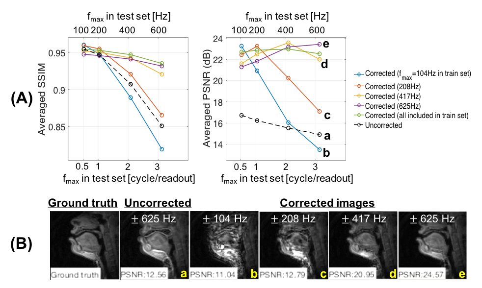
Figure 3(A) shows that the best performance is achieved when the training and test datasets share the same range of off-resonance. However, when severe off-resonance appears in the test data as fmax increases, the network trained with frequency range less than the fmax presented in the test data does not result in good performance, which is also observed in Figure 3(B). Network trained on all the training data with 4 different fmax was used for the rest.
Representative image frames are shown in Figure 4. The simulated blurring is seen most clearly at the lips, hard palate, and tongue boundary in the distorted image whereas sharper boundary can be observed in the image after correction.
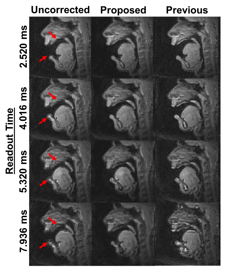
Figure 5 contains prospective results with long readouts. By visual inspection, the proposed method provides substantially improved depiction of air-tissue boundaries compared to a leading previous method.3
Conclusion
We demonstrate a simple and fast calibraionless CNN-based deblurring method for 1.5T spiral speech RT-MRI. The proposed network trained on simulated off-resonance images is effective at resolving off-resonance blurring at vocal tract tissue boundaries even with readouts 3-times longer than what is typically used today
Acknowledgements
This work was supported by NIH Grant R01DC007124 and NSF Grant 1514544.References
1. Block KT, Frahm J. Spiral imaging: a critical appraisal. J Magn Reson Imaging. 2005;21:657–668.
2. Meyer CH, Hu BS, Nishimura DG, Macovski A. Fast spiral coronary artery imaging. Magn Reson Med. 1992;28:202–213.
3. Lim Y, Lingala SG, Narayanan SS, Nayak KS. Dynamic off-resonance correction for spiral real-time MRI of speech. Magn Reson Med. 2018; https://doi.org/10.1002/mrm.27570
4. Man LC, Pauly JM, Macovski A. Multifrequency interpolation for fast off-resonance correction. Magn Reson Med. 1997;37:785–792.
5. Eigen D, Krishnan D, Fergus R. Restoring an image taken through a window covered with dirt or rain. In Proc of 2013 IEEE International Conf on Computer Vision. 2013. p. 633–640.
6. Dong C, Loy CC, He K, Tang X. Image Super-Resolution Using Deep Convolutional Networks. IEEE Trans Pattern Anal Mach Intell. 2016;38:295–307.
7. Zeng D, Shaikh J, Nishimura DG, Vasanawala SS, Cheng JY. Deep Learning Method for Non-Cartesian Off-resonance Artifact Correction. In Proc of the 26th Annual Meeting of ISMRM, Paris, France, 2018. Abstract 0428.
8. Abadi M et al. TensorFlow: a system for large‐scale machine learning. In Proc of the 12th USENIX conference on Operating Systems Design and Implementation, Savannah, GA, 2016. p. 265‐283.
9. Kingma DP, Ba J. Adam: a method for stochastic optimization. arXiv 2014:1412.6980.
Figures